It is here, finally, our optical tweezer setup mounted on a Andor Dragonfly. With the help of Impetux Optics and a generous FEDER grant from the spanish ministry/EC, we were able to assemble a unique combination of high-speed confocal imaging in 7 colors with optical force measurements and application.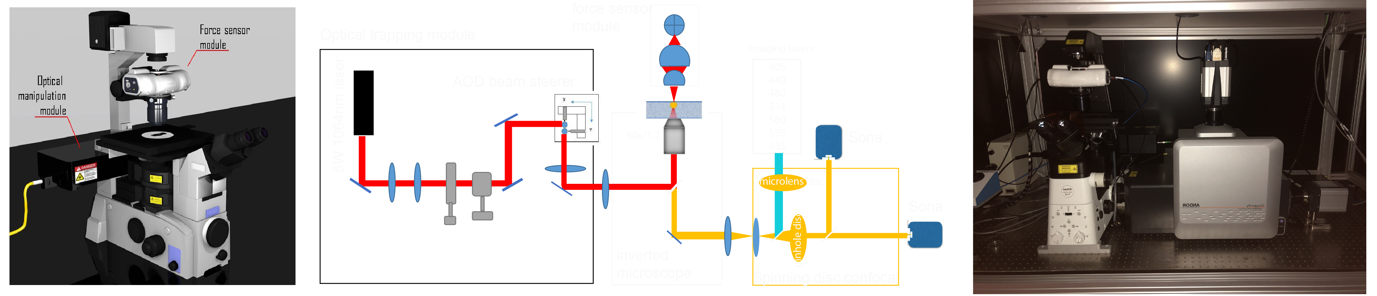

Optical tweezers is a non-invasive micromanipulation technique based on the accurate use of laser light momentum. These are capable of capturing, moving, pushing and rotating micron-sized particles thanks to the linear and angular momentum carried by photons. In Fig. 1, we sketch a highly focused laser beam upon interaction with a micro-sphere. The scattered light undergoes changes in momentum that result in restoring forces that maintain the particle captured within a small volume, which is so-called an optical trap.

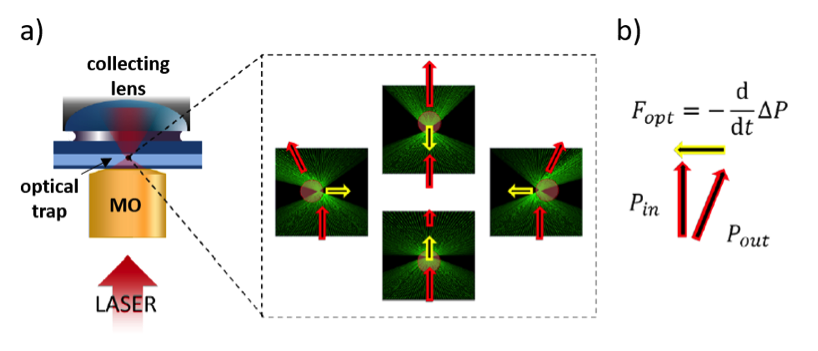
By the use of sophisticated light modulation techniques, such as acousto-optic deflectors (AOD), we can dynamically generate arrays of multiple optical traps to simultaneously trap different particles. Interestingly, we can detect the change in linear momentum to measure forces ranging from hundreds of femto-Newtons to hundreds of pico-Newtons. In cellular biology, forces governing a wide number of mechanical processes fall precisely in this range. This, together with the non-invasive nature of optical tweezers, enables quantitative force measurements in a wide number of experiments.

OPTICAL TWEEZERS FOR MECHANOTRANSDUCTION

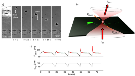
The newest toy in the hood! In our group, we are interested on how cells –and especially neurons- mechanically interact with their surroundings and execute vital functions such as proprioception and touch sensation. In order to investigate the mechanotransduction pathways that govern such functions at the cell scale, we make use of optical tweezers to locally perturb the cell membrane. As an example, a membrane tether pulling experiment on a HeLa cell is shown in Fig. 2a. A polystyrene, 3-mm microbead is trapped and brought against the cell membrane and a lipid tube, also known as tether, is extruded from the membrane. At time  the trap is turned off, so the tether brings the microbead back towards the membrane.

From this kind of experiments, we can perform localized increases in membrane tension on neurons (Fig. 2b) and assess important mechanical and information from it, as well as how a mechanical input is signaled along the cell through different ion flux pathways. In Fig. 2c, see a typical force curve obtained from a membrane tether extrusion experiment. The tether is elongated at increasing speeds to produce force peaks of increasing height. Subsequently, it is kept at constant length to wait for relaxation down to the static membrane tension.

OPTICAL TWEEZERS FOR intracellular force measurements and mechanical charazterisations

Here we present our protocol that appeared in the Journal of Visualized experiments 2021 by Frederic Catala and colleagues. Please don’t forget to cite this paper in cae you find the following documents helpful. This technique is still improving and capabilities are growing so keep an eye out to the twitter feed or the news pages for updates. The called out references refer to the numbers in the paper, so please check them out there.

Protocol

All protocols used have been approved by the Institutional Animal Care and Use Ethic Committee (PRBB-IACUEC) and implemented according to national and European regulations. All experiments were carried out in accordance with the principles of the 3Rs. Zebrafish (Danio rerio) were maintained as previously described.

1. Preparation of isolated primary embryonic zebrafish progenitor stem cells

1. Micropipette and agarose preparation
   NOTE: For a complete zebrafish embryo microinjection protocol, see reference⁴⁵.
   1. With a micropipette puller, pull a 1.0 mm glass capillary to obtain two needles⁴⁵. Store the unused needles in a 150 mm Petri dish attached to a playdough cushion or in an inside-out lab tape ring to protect the thin tip from damage during transport.
   2. Melt 1% ultrapure agarose in E3 (5 mM NaCl, 0.17 mM KCl, 0.33 mM CaCl₂, 0.33 mM MgSO₄) in a standard kitchen/lab microwave for 10 s. Heat the mix repeatedly for short periods of time (few seconds) until the agarose melts.
   3. When the agarose is completely melted, let it cool down briefly, and then pour it into a 10 cm Petri dish. Slowly add the triangular microinjection mold (see Table of Materials) on the top of the agarose avoiding the appearance of bubbles. Do not push the mold, ensuring it stays on the agarose surface.
   4. When the agarose solidifies completely, remove the triangular mold very slowly by exerting a gentle force to avoid any breaks in the agarose. The plate can be stored upside down at 4 °C for 2-4 weeks.
   5. 30 min before the microinjection, take the plate out of the fridge and add E3 prewarmed to 28 °C to let it stabilize at room temperature.
2. Injection mix preparation
   1. To prepare the injection mixture, dilute 1 µm microbeads (polystyrene, non-fluorescent) in 1:5 ratio in RNase free water.
      UPDATE: you may wish to passivate the microspheres such that they will not clog the needle and attach non-specifically to the intracellular structures and thus modulate the mechanical measurements.
   2. Prepare mRNA for transient expression of fluorescent markers or expression of recombinant gene constructs and/or co-injection of morpholino at the desired concentration.
      ​NOTE: A typical injection mixture for the co-injection of microbeads together with 100 pg of mRNA per embryo to label, for example, the nucleus with H2A-mCherry is: 1 µL of beads + 1 µL of mRNA (stock concentration is 1 µg/µL) + 2.5 µL of RNA free water + 0.5 µL of phenol red (stock solution 0.5%, phenol red is not mandatory; it is used for a better visualization of the injected drop but the non-labeled injection drop is also visible for an experienced experimenter). RNA injection can also be useful to select injected embryos. Fluorescent microbeads can be injected, instead of non-fluorescent, to visualize them.
3. Microinjection needle loading and calibration
   1. Turn on the microinjector using the Time-Gated option. This setting is very important to calibrate the injection volume properly. Set the gating time at approximately 500 ms.
   2. Load 3 µL of the injection mixture into the needle using a micro-loader pipette.
   3. Insert the needle into the micromanipulator and seal tightly. Check whether the micromanipulator is in a good position and has enough freedom to move in x-y direction on the injection plate.
   4. Measure the drop size using a micrometer slide (5 mm/100 divisions) with a drop of mineral oil on top⁴⁵ and ejecting a drop of the injection mix directly into the mineral oil.
   5. Crop the needle with sharp forceps at a steep angle to generate a sharp pointed tip. Adjust the drop size to 0.1 mm, corresponding to 0.5 nL of injected material.
      ​NOTE: If by cutting the needle, this volume is exceeded, it is recommended to redo the calibration procedure with a new needle. The gating time of the microinjector can be slightly adjusted to match the drop volume; however, short gating times correspond to a large needle diameter, which potentially damages the embryos.
4. Microinjection of zebrafish embryos at one-cell stage
   1. Collect zebrafish embryos shortly after fertilization for microinjection of the bead mixture directly into the one-cell (zygote) stage embryo before the first cell division occurs.
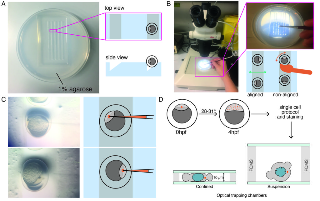
      NOTE: This ensures proper distribution of microspheres and a high enough yield of isolated blastomeres with at least one microsphere per cell at later developmental stages in which experiments are performed (blastula-gastrula stage). Indentation experiments can still be performed if there are two spheres within the cell, but cells that have no beads should be excluded (even though indentation without spheres is possible). AB wildtype strains were used in this protocol, but any other strain, e.g., TL can be used.
   2. Place one-cell stage embryos (zygote) in a prewarmed triangular-shaped 1% agarose mold, as shown in Figure 1A, using a plastic Pasteur pipette.
   3. Remove extra medium with the same pipette to avoid the embryos floating around. Gently push the embryos into the triangular mold via a brush. Keep some space in between embryos to facilitate the correct orientation (Figure 1B).
   4. Gently align the embryos with a brush so that the embryos are oriented laterally, with the one cell of the zygote being clearly visible, as shown in Figure 1B. An ideal orientation for microinjection is reached when the one cell of the embryo is facing the needle direction (injection via the animal pole of the embryo) or in the opposite way facing the yolk cell (injection via the vegetal pole of the embryo), as shown in Figure 1C.
   5. Hold the dish with one hand and use the other hand to position the needle tip using the micromanipulator controller. Lower the needle tip toward the embryos.
   6. Pierce the chorion and enter the one-cell embryo with the needle while monitoring the procedure through the stereomicroscope. Ensure correct placement of the needle and, after injecting, the correct location of the injected drop as shown in Figure 1C.
   7. Repeat for all embryos: move the needle up, slide the dish with the embryos until the next embryo is centered, lower the needle, and inject it.
   8. Once the entire set of embryos is injected, remove the embryos from the agarose mold/Petri dish by flushing some E3 and put them in a new Petri dish using a plastic Pasteur pipette. It is recommended to place sufficient media on the injection plate to avoid drying out of embryos during the microinjection procedure.
   9. Repeat the procedure until the desired number of embryos is injected. Embryos must be at one cell stage to ensure maximal and homogeneous spreading of the beads.
      NOTE: This procedure is optimized for early blastula embryos and likely needs to be optimized if different developmental stages are to be investigated.
   10. Place the injected embryos inside an incubator at 28-31 °C for approximately 4 h or until the desired stage (Figure 1D) before proceeding with the protocol for primary cell culture.
       ​NOTE: Optionally, let the embryos develop beyond the blastula stage (or desired measurement time point) to ensure survival and rule out toxicity artifacts. At larval stages, mount anesthetized larvae with tricaine in 0.75% agarose and image the distribution of microspheres in various tissues. To make a stock solution, mix: 400 mg of tricaine powder in 97.9 mL of distilled water, approximately 2.1 mL of 1 M TRIS-base (pH 9), and adjust to pH 7. This solution can be stored at 4 °C. To use tricaine as an anesthetic, dilute 4.2 mL of stock solution in 100 mL of egg’s medium (or desired media); in this case, E3 was used. Consult reference⁴⁶ for details.
       

2. Single-cell preparation and staining

1. Place the sphere stage embryos (4 hpf, hours post fertilization) in a glass dish using a plastic Pasteur pipette. Select the embryos that are positive for the signal of the injected beads, and that express the fluorescent protein in case of mRNA injection. Some embryos might show high bead clustering and can be excluded.
   1. Manually dechorionate the embryos using forceps. Transfer approximately 10-15 embryos to 1.5 mL reaction containers using a glass Pasteur pipette.
      NOTE: When the embryos are dechorionated, they attach to the plastic, and the use of glassware is required. As an alternative to the glass plate, a plastic Petri dish with a thin layer of 1% agarose can be used. Manual dechorionation should be preferred over enzymatic Pronase treatment to prevent proteolytic damage to cell surface proteins and potential changes in mechanical cell and tissue properties, preventing extended recovery times⁴⁷.
2. Remove the E3 media and add 500 µL of pre-warmed CO₂-independent tissue culture medium (DMEM-F12; with L-glutamine and 15 mM HEPES, without sodium bicarbonate and phenol red supplemented with 10 units penicillin and 10 mg/L streptomycin).
   NOTE: Do not use CO₂-dependent media unless a microscope incubator is used. The use of, e.g., RPMI in carbonate-buffered conditions cause changes in the media’s pH and can affect cell survival. Another key aspect is to avoid culture media that contain serum. Serum may contain Lysophosphatidic acid (LPA), a potent activator of the Rho/ROCK pathway, capable of controlling cellular contractility and motility in progenitor stem cells⁶. The osmolarity of the medium should be maintained at 300 mOsm to avoid osmotic challenges that could interfere with nuclear morphology or mechanics¹².
3. Manually dissociate cells by gently shaking the tube. Ensure that the contents of the tube become turbid with no big chunks visible by the eye. Avoid the formation of bubbles to minimize the damage and loss of cells.
4. Centrifuge at 200 x g for 3 min. The pellet must be clearly visible.
5. Remove the supernatant and follow one of the steps detailed below.
   1. If no staining is needed, add 500 µL of DMEM. Gently resuspend with a 200 µL pipette by targeting a liquid jet onto the pellet. Do not exert excessive shear force onto the cells. Foaming indicates damage to the cells.
   2. For labeling the nucleus with DNA dyes such as Hoechst, mix 0.5 µL of DNA-Hoechst (stock 2 mg/mL) in 1,000 µL of DMEM to obtain 1 µg/mL of final concentration. Add 500 µL of this staining solution to the cells and resuspend gently. Incubate for 7 min in the dark.
   3. To stain the cells with a fluorescent chemical calcium indicator Calbryte-520, add Calbryte-520 to a 5 µM concentration in DMEM. Incubate for 20 min in the dark.
      NOTE: The protocols indicated in steps 2.5.2 and 2.5.3 have been optimized for these specific products. Other staining can be performed using the protocols indicated by the manufacturer.
6. Centrifuge again using the same settings as in step 2.4; remove the supernatant, and gently resuspend the cells (to avoid the formation of clusters) in 50 µL of DMEM for samples in suspension or 20 µL of DMEM for cells in confinement.

3. Preparation of optical trapping chambers using polydimethylsiloxane (PDMS) spacing

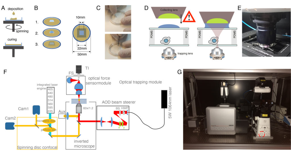
NOTE: Optical force measurements based on light momentum detection require the capture of all the light emerging from the optical traps⁴⁰. For the robustness of the invariant calibration factor α (pN/V), the light distribution at the back focal plane (BFP) of the optical force sensor must bear an accurate correspondence to the photon momentum. This determines the distance from the surface of the collecting lens to the trapping plane to approximately 2 mm, which is the maximum height of the optical trapping chambers.

1. PDMS spin-coating of #1.5 glass bottom dishes.
   NOTE: The following recipe is provided for approximately 40 dishes. The resulting microchamber will have different heights depending on whether experiments are to be conducted on suspended or confined cells (Figure 1D).
   1. Mix 9 mL of the base polymer PDMS and 1 mL of PDMS curing agent in a 50 mL conical tube. Mix the two products actively to ensure proper distribution of the curing agent.
   2. Degas the mixture to avoid bubbles using a vacuum pump. Introduce the conical tube in a vacuum bottle and evacuate the chamber. Wait until no bubbles are present in the mixture.
      NOTE: Open the vacuum slowly to prevent foaming and spills of the PDMS out of the falcon tube.
   3. Place the glass bottom dish on the spin-coater chuck (Figure 2A). Be gentle not to scratch, fingerprint, or get the dish dirty. Protect the spin-coater box from PDMS leaks with aluminum foil.
   4. For OT chambers for experiments on cells in suspension, add approximately 250 µL of PDMS mixture at the center of the bottom dish and spin it at 750 rpm for 1 min. The height of the PDMS layer will be 50 µm approximately⁴⁸.
   5. For OT chambers for experiments on confined cells, add a small drop of PDMS (approximately 50 µL) and spin it at 4,000 rpm for 5 min. The height of the PDMS layer will be 10 µm approximately. For a detailed protocol on how to obtain different PDMS thicknesses, see reference⁴⁸.
   6. Cure the PDMS-coated glass-bottom dishes at 70 °C for 1 h.
   7. Cut a 1 x 1 cm square onto the PDMS layer with a scalpel and peel it off with tweezers (Figure 2C). In the case of confined cells, wash PDMS debris with isopropanol.
2. Chamber coating for experiments with lightly attached cells in suspension
   1. Add 100 µL of Concanavalin A (ConA) at 0.5 mg/mL to cover the entire surface of the square cavity and let it incubate for 30 min.
      NOTE: ConA is a lectin that binds to cell surface sugars and couples individual cells onto the coverglass surface.
   2. Remove the ConA drop and rinse the surface carefully with DMEM medium without scratching the ConA treated surface.
   3. Add 30 µL of the previously prepared sample (step 2.6) into the well and gently resuspend to get rid of any cell clusters.
   4. Close the cavity by gently placing a 22 x 22 mm #1.5 cover glass on top of the PDMS rims (avoid letting it fall abruptly, use forceps if possible, Figure 2B,C).
      NOTE: Any coverslip thickness would work for the upper glass cover (the collecting lens has a working distance of 2 mm).
3. Chamber preparation for experiments with cells in confinement
   1. Put a 10 µL drop of solution containing cells (step 2.6) into the square cavity (Figure 2B).
   2. Very gently, sandwich the sample with a 22 x 22 mm cover glass such that the drop spreads in the entire area and no bubbles are observed. Again, it is convenient to use forceps, as shown in Figure 2C, to prevent the cover glass from falling abruptly.

4. Alternative options for OT chamber spacing

NOTE: These steps can be followed if no microfabrication workshop or spin coater is available.

1. Chamber preparation for experiments with cells in suspension
   NOTE: In case no spin coater is available, a spacer can be made using normal, double-sided scotch tape (approximately 100 µm in height).
   1. Cut a piece of double-sided scotch tape with an approximately 10 cm x 10 cm square hole in the center (same dimensions as in PDMS, Figure 2B).
   2. Remove one of the protective layers of the tape by peeling it off and place the uncovered side of the tape in the center of a #1.5 H glass-bottom dish. Press gently to get all the surface adhered to the glass while avoiding air bubbles, and then remove the remaining protective layer of the tape by peeling it off.
   3. Follow the instructions in step 3.2.
2. Chamber preparation for experiments with cells in confinement
   NOTE: To precisely confine cells, monodisperse microparticles with a known diameter can be used as spacers between the two cover glasses.
   1. Add 10 µm polystyrene beads to suspended cells at a concentration of 10⁴ beads/µL.
   2. Put a 10 µL drop of solution containing cells and beads on a 22 x 60 mm cover glass.
   3. Very gently, sandwich the sample with another 22 x 60 mm cover glass such that the drop spreads in the entire area and no bubbles are observed. To position the upper cover glass gently (avoid that it falls down abruptly), it is convenient to use forceps.
   4. As the sample can dry out, it is recommended to perform the preparation swiftly.

5. Setting up the optical trap for intracellular measurements

NOTE: The following steps are optimized for a commercial optical tweezers platform comprising an optical micromanipulation module based on acousto-optic deflection (AOD) and an optical force sensor based on direct detection of light momentum changes (Figure 2, reference^12,40,49). Details and optical components of the set-up can be found in Figure 2F. To observe force-induced deformation during the optical tweezer manipulations, a Nipkow spinning-disk confocal microscope is coupled into the left port of the inverted microscope for dual color fluorescence imaging. Without the lack of generality, this protocol can be applied with any dynamic OTs system equipped with direct force measurements based on light momentum detection. Detailed step-by-step procedures are available to construct homebuilt optical gradient traps for in vivo applications⁵⁰. Those based on AOD modulation stand out for eventual experiments with multiple traps and fast measurements^51,52. Several protocols to construct a light-momentum based instrument exist in the literature^36,39,40,53, and any other imaging modality (differential interference contrast, widefield fluorescence, etc.) can be employed.

1. Optical tweezers start-up
   1. In order to optimize for the output power stability, turn on the laser at considerably high power (e.g., 3 W) at least 30 min before the experiment.
   2. Turn on the electronics module of the optical micromanipulation and force measurement units.
      NOTE: Apply all laser safety measures and only use equipment approved by the institutional board. Never use the eyepieces of the optical microscope when the laser is on. Always use approved IR protection goggles (OD7 in the 950-1080 nm range), block the IR laser light with the shutter in the epifluorescence port 2, and do not execute the optical trapping software until finishing the optical force sensor alignment after step 5.3. In general, do not use a highly reflective sample, as the back-reflection could cause damage to the laser.
   3. Control the trap power with the rotating HWP (Figure 2F) at the entrance of the optical micromanipulation module.
      NOTE: The commercial optical micromanipulation module used in this protocol already incorporates this feature. For homebuilt optical trapping systems, integrate this tool for power control so that higher and more stable laser powers can be used.
2. Use an empty microchamber for calibration
   1. Cut a 1 x 1 cm square onto a double-sided scotch tape and attach it onto a 1 mm thick microscope slide.
   2. Add water into the square and close it from the top with a #1.5 cover glass (22 x 22 mm). Adding a slightly higher volume of water, e.g., 30-40 µL is advised to avoid bubbles inside the covered chamber. Wipe the calibration chamber gently in case of water spilling out of it.
3. Alignment of the optical force sensor
   1. Put a droplet of water on the 60x/1.2 water immersion objective. Place the calibration chamber on the stage with the #1.5 cover glass facing the objective. Focus onto the lower surface, where the cell samples will eventually be.
   2. Add a droplet of immersion oil on top of the upper glass slide covering the sample (Figure 2D). Lower the collecting lens of the force sensor unit carefully until it contacts the oil droplet.
      NOTE: The droplet must be large enough so that it covers the whole lens that collects the laser light emerging from the traps. Usually, 200 µL is sufficient to cover the entire surface and provide a stable immersion contact. Be conservative and avoid overfilling as it might leak into the sample.
   3. Following the manufacturer’s protocol for the optical force sensor alignment, look at the sample plane image on the auxiliary camera that will be used to position the OTs (AUX, Figure 2F). Very gently, lower the optical force sensor until the field stop (FS, Figure 2F-G) appears conjugated onto the sample plane. This will ensure proper direct force measurements from sample-invariant detection of light momentum changes⁴⁰.
      NOTE: Close the FS enough so that its image becomes smaller than the field of view (FOV), hence, visible. Be extra careful and do not push the collecting lens of the optical force sensor against the sample. The vertical position of the optical force sensor can alternatively be determined from analysis of the trapping light distribution at the BFP for light cones with defined numerical aperture (NA).
   4. Ensure that there are no air bubbles in the oil droplet; these can directly affect the force measurements. To check for air bubbles, put the Bertrand lens in place (BL, Figure 2G) and observe the imaging path through the eyepiece. If any dirt or air bubbles are visible or more oil is needed (Figure S1A), clean the lens and chamber with dust-free lens tissue and repeat the procedure in steps 5.3.2 and 5.3.3. An unobstructed optical path is depicted in Figure S1B.
   5. Using the lateral screws placed on the holder of the optical force sensor, center the FS into the FOV. For accuracy, open the FS so that it almost fills the FOV visible on the auxiliary camera (AUX, Figure 2F).

6. Optical tweezer optimization

NOTE: The direct force measurement relies solely on the change of light momentum arising from the force exerted onto the trapped particle, and thus, in contrast to indirect methods, trap stiffness does not need to be calibrated prior to each experiment. The instrument-specific conversion of deflection/force factor (α; pN/V, reference⁴¹) is calibrated by the manufacturer and is thus experiment invariant. However, because the laser spot is manipulated over an area of 70 µm x 70 µm, steps 6.2-6.5 are critical to ensure optimal trapping and power stability. The following steps are supplied in the manufacturer software so that the OTs get optimized over the working area in a semi-automatic way.

1. Launch the OTs software and the acquisition software for camera AUX.
2. Subtract the initial voltage baseline by clicking on the Step 1: Electronics Offset step in the System Calibration submenu of the optical tweezers driving software.
3. To perform trap power flattening across the OT working area, set the trap power to half of its maximum by rotating the HWP accordingly. Do not change the trap power by changing the laser output, but with the rotating HWP (Figure 2F). Click on Step 2: Power to initiate the automated routine for trap power flattening.
   NOTE: This is a critical step to compensate for variation of the trap power across the OTs working area (Figure S1D). A successful routine brings trap power variation down to 2% across the OTs working area and converges after 2 min.
4. To perform trap position calibration, remove the IR filter so that the light from the laser is visible on the camera. Find the IR spot by setting the image plane focused onto the lower surface of the microchamber. Obtain the smallest IR spot possible by tuning the image plane (objective position) and the histogram contrast in camera AUX acquisition software. If needed, reduce the power of the optical trap by rotating the HWP (Figure 2F). Click on Step 3: Position to start the automated routine or trap positioning calibration.
   NOTE: This routine enables the precise correspondence of the OT’s position coordinates in camera AUX to the AOD steering angles. A successful routine generates the angle-to-position mapping in several seconds.
5. Initial momentum compensation
   NOTE: The movement of the optical trap across the sample causes variations in the light-momentum distribution at the BFP (Figure S1E, F). This leads to force-independent signal changes related to laser position over the working area, even though the trap power has been flattened as in step 6.3. The consequence is a variation in force baseline due to position (independent of an actual force acting on the optically-trapped bead) that needs to be corrected prior to each experiment.
   1. Set the trap power that will be used in the experiments, by rotating the HWP (Figure 2F).
   2. Click on the Global Offset option in the Tools submenu. This will open the Offset Cancel assistant of the optical tweezers software that corrects the initial momentum baseline.
   3. Click on Offset | Compensate to correct the position-variant initial momentum.
      NOTE: If no modification affects the optical path during the ongoing weeks, the trap power flattening (step 6.3) and position (step 6.4) maps will remain invariant. We hence recommend to always use the same combination of optical elements (dichroic mirrors, filters, etc.) that may affect the laser trap path or to carry out a new trap power flattening routine. Regarding the initial momentum compensation (step 6.5), the manufacturer of the OTs platform provides an on-the-fly calibration that must be changed for every new trapping power and experimental session. Steps 6.3 and 6.4 must be carried out on the empty calibration slide described in step 5.2. In a sample containing cells or other objects, step 6.5 should be carried out free of objects that may alter light scattering in the OTs working area.
6. Optionally, trap a microsphere and move the trap at a known velocity while recording the force signal. For example, set the trap to perform a triangular oscillation: the recorded force signal will be a square signal.
   NOTE: The force value should increase linearly with the velocity, according to the drag force acting on the bead. This test serves as a positive control that force measurements are being undertaken correctly³⁸. Alternatively, the optical force sensor can be used to obtain the optical trapping stiffness, κ [pN/µm], and the position calibration factor, β [µm/V], from power spectral analysis³⁵. Under correct alignment, the invariant calibration factor provided by the manufacturer is α = κ·β [pN/V].
   1. Initiate a real time force reading by clicking on Plot 1 in the Measures submenu in the manufacturer software. This will provide a reading of the current optical trapping force and power.
   2. Open the Oscillation Parameters dialog from the Tools submenu. Set a triangular-space waveform shape in the Shape and Type selector rings, respectively. As an example, set an amplitude of 10 µm and a frequency of 3 Hz. This will result in a viscous force of approximately 1 pN onto a microbead with a diameter of 1 µm³⁸.
   3. On the camera’s AUX window, right-click on the microbead and select Start Oscillating. The force reading will become a square force signal with plateaus at ±1 pN.
   4. Right-click on the microbead and select Stop Oscillating.

7. Spinning disk confocal microscopy

1. Turn on the spinning-disk confocal microscope and accessory equipment, the integrated laser engines, and the acquisition cameras.
2. Launch the imaging software.
3. Set imaging channels for Hoechst staining of the nucleus and GFP for the cell plasma membrane.
   1. Activate the 405 nm and 488 nm excitation lasers lines.
   2. Add a multiband dichroic to reflect the excitation to the sample and that allows emitted light to pass to the cameras.
   3. Split the fluorescence emission with a 500 nm long pass edge dichroic mirror.
   4. Use the DAPI/BFP (~445 nm) and GFP (~521 nm) emission filters in front of the two acquisition cameras, respectively. Refer to Figure 2F,G.
   5. Set the exposure time to 100 ms for each channel.
   6. Set laser emission to obtain a power of 5 mW at the sample plane. To measure the power, use a commercial power meter.
4. Set the imaging protocol. To avoid spectral bleedthrough from the Hoechst channel into the GFP channel, the two dyes need to be imaged sequentially.
   ​NOTE: If a hardware synchronization exists between the AODs of the optical trap and the camera acquisition, make sure that the trigger polarity is set up correctly. If in doubt, consult your facility manager or microscope manufacturer.

8. Performing the nucleus indentation experiments

NOTE: Always turn off the optical traps-both using software and closing the shutter on epifluorescence port 2-when lifting the force sensor module and changing the sample. If not, serious damage to optical elements and the experimenter could occur. Be careful with the lateral distance between lens holder and bottom dish edge when looking for cells to avoid bumping the lens into the stage/culture dish (Figure 2).

1. Place the sample in the microscope and follow step 5.3 of this protocol.
2. Using the rotating HWP (Figure 2F), set the trap power to 200 mW as a starting value if the stiffness of the nucleus or intracellular structure investigated is not known. Translate the OTs working area (using the microscope stage) to a place free of cells in order to compensate for the initial momentum baseline through step 6.5.
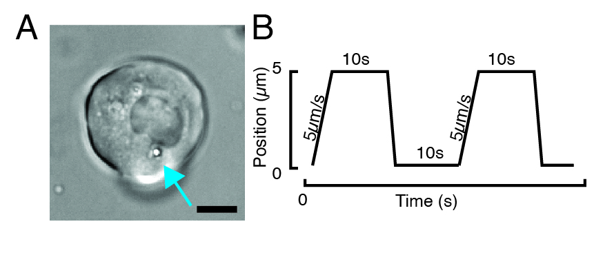
   NOTE: Depending on the stiffness of the subcellular structure, the trap power value should be adjusted to lower or higher values to obtain a similar indentation depth.
3. Using the microscope stage software controller, look for a cell with one or two beads through transmitted brightfield microscopy (Figure 3A).
4. Define a trap trajectory.
   1. Open the Trajectory dialog in the Tools submenu and choose Displacement in the Trajectory Type selector ring.
   2. In the numerical sheet, write the displacement and time of each subsequent trajectory step. Here are two examples.
   3. For a stress relaxation experiment, program trapezoidal loads, as shown in Figure 3B. In Table S1, two trapezoidal indentations were applied with a travel distance of 5 µm; velocity of 5 µm/s; waiting time before retraction: 10 s.
   4. For a repetitive indentation experiment at a constant velocity to obtain a triangular routine without dwell time on the nucleus, set the trajectory amplitude, e.g., 5 µm, and the time for the step, e.g., 2 s for a velocity of 2.5 µm/s. In Table S2, this is applied eight times at the same velocity.
      NOTE: These values need to be determined for each cell type and experiment, but the following parameters of a trapezoidal routine capture the most important dynamics in the experiment presented here. The waiting time should be sufficient for the nucleus to show its complete stress relaxation after indentation
5. Trapping a microsphere
   1. Set the image plane slightly above the bead with the microscope stage software controller.
   2. Activate traps using the OTs software and click on the bead in the camera AUX imaging window (calibrated following step 6.4). Successful confinement of the bead by the optical trap will strongly reduce the motion of the bead.
   3. Click-and-drag the bead across the cytoplasm and place it at a distance of ~2 µm from the nuclear envelope (Figure 3A). Make sure that the trajectory is set so that the bead indentation is perpendicular to the nuclear membrane.
6. Optionally, if needed for position measurements of the bead relative to the trap, scan the trap across the bead to determine the trapping stiffness, k [pN/µm]⁵⁴, thereby Δx_bead = –F/k (see Discussion). The optical micromanipulation module used in this protocol has a built-in routine for this purpose.
   1. Open the Particle Scan dialog in the Tools submenu.
   2. Select the trap you want to scan and High Frequency as the Scanning Method. Select the direction (x or y) of the indentation trajectory for the bead scanning measurement.
   3. A window will appear with the measurement of the trapping stiffness. In the graph, drag the two cursors to select the linear trapping area corresponding to F = –kx. The linear fit to the selected data portion will be refreshed automatically.
      NOTE: Set the initial position of the bead far from the cell membrane (~5 µm), as light-momentum deflections at the medium-cell interface affect the appropriateness of force measurements. If the nucleus is located too close to the cell membrane, try to indent the nucleus from the opposite site. Discard the cell if not possible.
7. Start image acquisition by clicking on the acquisition button in the imaging software.
8. Start trap position and force measurement data saving by clicking on Data | Save in the real time force reading window (opened as in step. 6.6.1).
   NOTE: The optical trap is equipped with a trigger input which can be connected to the timing output of the camera. Thus, image and force data are hardware-synchronized and the electronic is able to map the trap cycles with the number of frames of the images during the acquisition.
9. Initiate the previously loaded trajectory by right-clicking on the bead and selecting Start Trajectory.
10. Wait until the trajectory is finished and the system stabilizes.
11. Stop trap force measurement data saving. A data saving dialog will pop up.
    NOTE: To optimize data storage, data can be decimated by selecting the decimating parameter in this dialog (10, 100, or 1000).
12. Stop image acquisition and plot the results in the postprocessing software of the user’s choice.
13. If the microsphere is lost during the routine and the nucleus cannot be indented (Figure S2), discard the measurement and increase the power. Note that step 6.5 must be repeated. In our hands, at least 95% of the routines are successfully completed without losing the bead from the trap.

Representative Results

Microinjection of trapping beads:
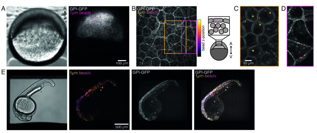
Microspheres injected into the one-cell zebrafish embryo spread over the entire animal cap during morphogenesis. For a clearer visualization, we repeated the injection protocol with red fluorescent microbeads and took volumetric images with our confocal microscope at different developmental stages. In Figure 4A–D, injected beads are visualized in the cytoplasm of progenitor stem cells in vivo at 5 hfp. Later on, microspheres appeared spread over the whole embryo at 24 hpf (Figure 4E). Embryos at both stages developed normally and survival rates were comparable with control non-injected or mock-injected embryos (see Figure S3). This is consistent with other studies that report unperturbed survival of bead-injected zebrafish up to 5 days post fertilization⁵⁵.

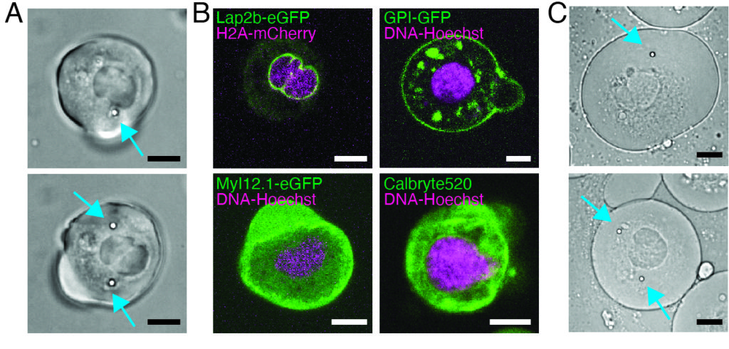
Our spinning-disk confocal microscope is compatible with multi-channel fluorescence microcopy. In Figure 5A, we show isolated stem cells with one or two beads in the cytoplasm. Multiple fluorescent labels can be used to investigate different aspects of the cell (Figure 5B). Nuclear morphology can be tracked with a Hoechst dye or using a H2A::mCherry mRNA expression, while inner nuclear membrane can be analyzed with Lap2b-eGFP¹². Dynamics of the actomyosin cortex, as well as intracellular calcium levels, can be observed with a My12.1::eGFP transgenic line⁵⁶ and Calbryte-520 incubation, respectively. The protocol that has been described here aims to compare cell nucleus mechanics of immobilized wildtype cells on adhesive substrates (later referred to as suspension) and in mechanical confinement. Isolated stem cells confined in microchambers of 10 µm height exhibited partial unfolding of the inner nuclear membrane (INM) and a subsequent increase in actomyosin contractility¹². In Figure 5C, confined cells with one or two beads in the cytoplasm are shown. Successful confinement will be visible via flattened, expanded cells with a wider cross section of the nucleus. The nuclear membrane is further unfolded in confined cells and should appear smoothened out in comparison to cells in suspension (Figure 5C).

Force-time and force-deformation analysis
The analysis of the obtained results strongly depends on the investigated specimen and the question of interest and thus they cannot be generalized here. As an example, a common way to analyze indentation measurement is to extract a Young’s modulus by fitting a modified Hertz model to the force-indentation data⁵⁷. However, the assumption for such a treatment needs to be carefully assessed and might not always be properly justified (such as the investigated structure being isotropic, homogenous, with linear elasticity and indentations being smaller than the bead radius). We thus only consider model independent measurements here that allow the mechanical behavior of the investigated structure to be compared among different experimental scenarios.

As a starting point, measuring the slope of the force-displacement curve at a certain indentation depth provides a measure of a model independent structural stiffness⁵⁸ of the nucleus. This value can then be collected from multiple samples and compared between varying experimental settings and sample perturbations.

Indentation measurement
In the following lines, we focus on the mechanical response of the cell nucleus during cell deformation in confinement. Experiments in step 8 of this protocol typically lead to force peaks of up to 200 pN for indentation depths of approximately 2-3 µm. However, these values can be largely different, depending on the cell type and experimental conditions, with softer nuclei leading to lower force for a given indentation. It is thereby needed to accurately measure the nuclear deformation, together with force, for an accurate mechanical characterization of the cell nucleus. In this section, we will obtain the cell nuclear stiffness from representative force indentation measurements.

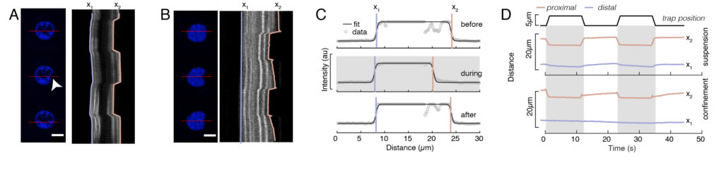
In Figure 6, we show the deformations of the distal and proximal sides of a nucleus in a suspended and confined cell. A rich mechanical behavior can be observed. In a typical suspended cell on an adhesive substrate, the nucleus was strongly indented by the bead, but also slightly displaced upon repetitive pushing events. We measured the bead indentation onto the nucleus by analyzing the kymographs obtained from fluorescence imaging of Hoechst-stained cell nuclei. Kymographs were easily computed using Fiji’s Multi Kymograph plugin along the indentation direction (Figure 6A,B) and imported into Matlab (Version 2021, Mathworks) for further processing. A step function was fitted to the raw intensity profile with the aim to track the delimiting edges of the nucleus along the trajectory of the indentation routine. As can be seen, it bears accurate information on the nuclear change in shape (Figure 6 and Figure S2). We used the following double-sigmoid curve as an analytical version of a step function:

         (Equation 1)

Here, x₁ and x₂ denote the distal and proximal edges of the nucleus, while A and B are the maximum and background gray values of the blue channel (Hoechst dye) of the image (Figure 6B). The edge width has been considered (e₀ = 0.25 mm). While the indented, proximal nucleus edge (x₂) followed the trajectory applied by the optical trap routine after the microsphere-nucleus contact, the opposite, distal edge (x₁) displays relaxation dynamics as expected for a viscoelastic material such as the cytoplasm (Figure 6D). In contrast, nuclei in cells confined in 10 µm high microchambers do not exhibit such translocation behavior of the nucleus upon indentation within the cell (Figure 6B,D). Also shown in Figure 6D, the rear edges of the nuclei remains unaltered by the bead pushing from the proximal side, most likely due to stronger forces arising from cell contractility and friction acting against the indentation force. In order to get the correct deformation depth, the displacement x1 was subtracted from the indented measure x2: Δx = x₂ – x₁ (see also Figure 6D).

Force data analysis
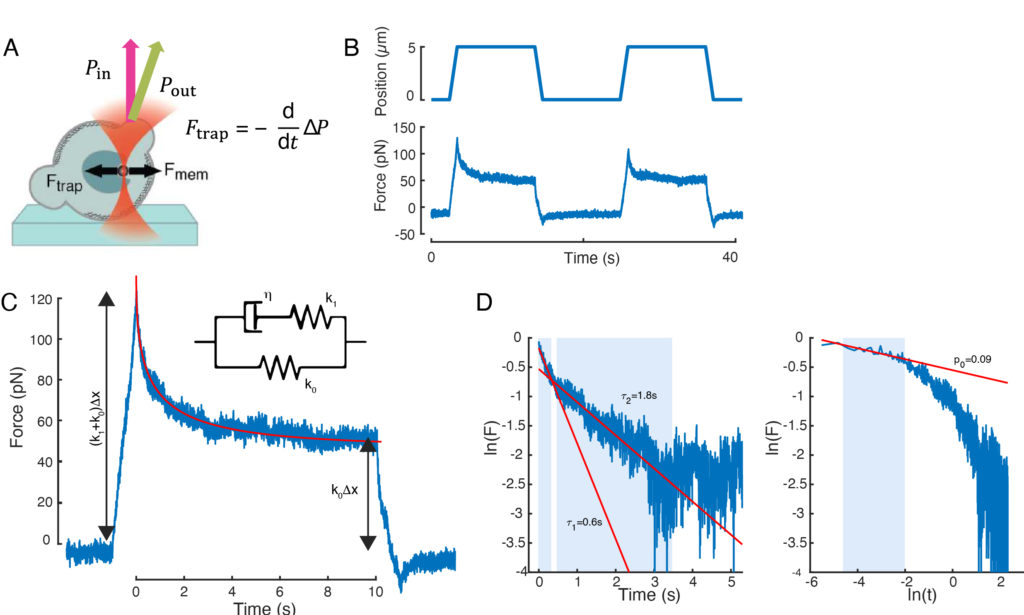
The force causing nuclear deformation was measured from the change in light momentum originated at the optically-trapped microbead (Figure 7A). The force upon applying trapezoidal trajectories (step 8.4.3, Figure 7B) initially increased linearly until the trap stopped moving, but then relaxed to a steady state value. This behavior indicated a viscoelastic material exhibiting loss and storage moduli. Right after the indentation event, the force reached a peak value, F_p, followed by a stress relaxation (Figure 7C):

          (Equation 2)

where F₀ is the stored force for the elastic component and f(t) is a dimension-less relaxation function. We have analyzed this behavior in three ways:

1. Considering a standard linear solid with an exponential stress relaxation, i.e., f(t) = e^–t/τ, schematically represented in Figure 7C inset.

2. Using a general, double-exponential decay:
F(t) = A + B₁e^-t/τ₁ + B₂e^-t/τ₂.

3. Using a power law followed by an exponential decay⁵⁹:
f(t) = t^-pe^-t/τ, fitted in Figure 7C.

While the fit for model 1 can be carried out straightforwardly, we recommend to estimate the initial guesses for (τ₁, τ₂) and (p, τ) for models 2 and 3, respectively. This can be performed, respectively, by fitting lines onto the data in logarithmic-versus-linear (Figure 7D, left) and logarithmic-versus-logarithmic (Figure 7D, right) scales. Table S3 summarizes the results for the example analyzed in Figure 7. In the following section, we will consider the combination of a power law and an exponential law for the characterization of the cell nucleus mechanics.

Force displacement relation
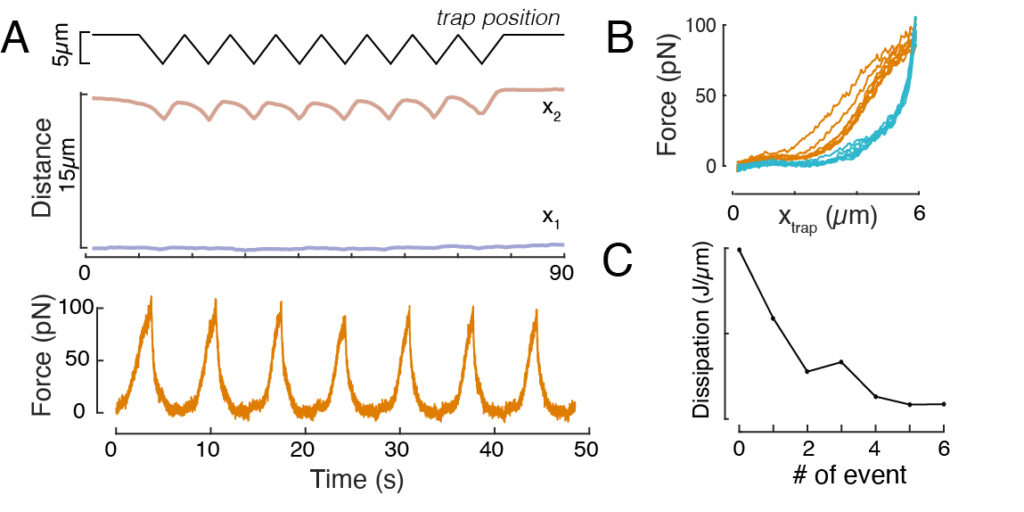
Likewise, the described experimental set-up can be used to obtain the force-displacement relation of multiple indentation events. By performing triangular routines (step 8.4.4, Figure 8A), it is possible to relate the force to the deformation and plot a force-indentation curve. An exemplary outcome is shown in Figure 8B, in which a flat baseline smoothly changed slope once the bead got into contact with the nucleus. Identifying the true contact point in the noisy data is a challenge, and care has to be taken to see whether the contact region is fit to elastic models⁶⁰. In this particular experiment, it could also be seen that the subsequent indentations result in curves with deeper contact points, indicative for too slow nuclear shape recovery after bead retraction and a change in the hysteretic cycle defined by the nucleus viscoelastic material properties (Figure 8C). Thus, the researcher should be aware if this happens and incorporate this into the analytical pipeline, or restrict the number of subsequent measurements such that this effect does not modify the measurement.

Nucleus mechanics in cells in suspension and under 10 µm confinement
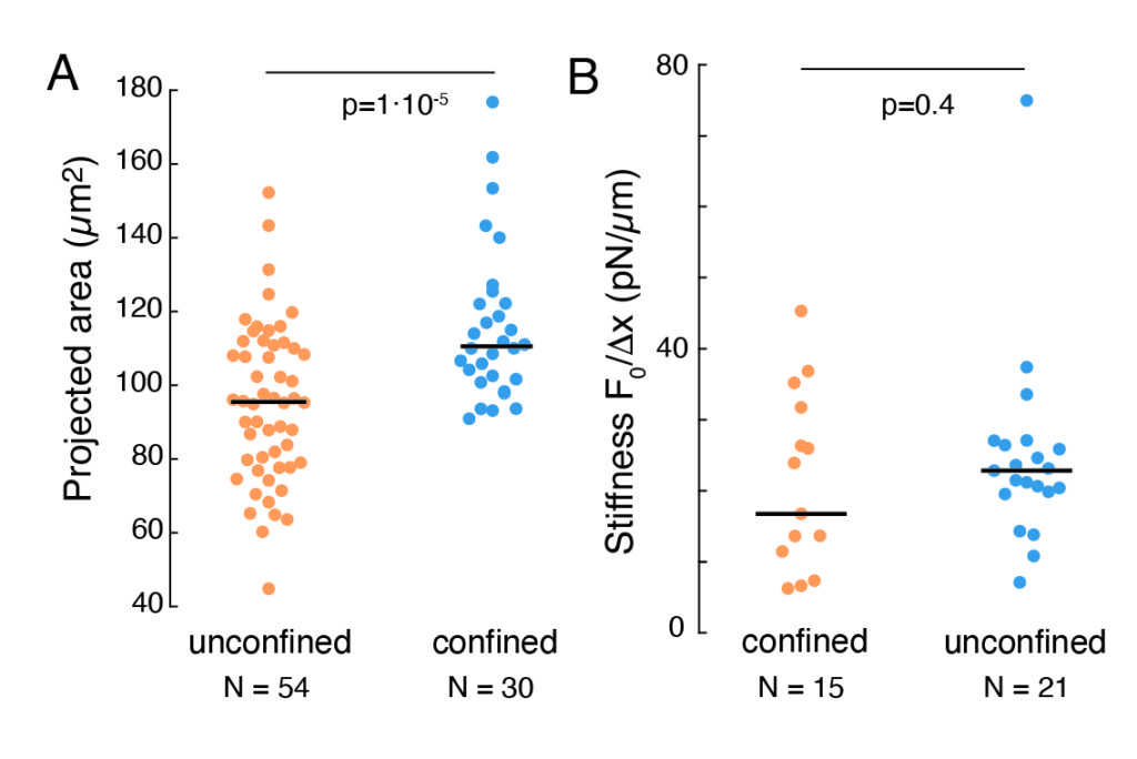
The aforementioned approach was used to analyze the dynamics of nucleus stress relaxation in suspended cells on adhesive substrates and confined cells. Our results show that the confinement results in an expansion of the projected area (Figure 9A), but insignificant change in nuclear stiffness (Figure 9B). We measured similar relaxation with τ = 6.08 ± 1.1 s (unconfined) and τ = 4.00 ± 0.6 s (confinement), which indicates fast viscoelastic dissipation, followed by a stored force value that corresponds to the elastic modulus of the nucleus. In order to account for experimental variations, which may be produced by different initial conditions in the indentation routines, measured stored forces were normalized to the indentation depth, as . This parameter accounts for the nucleus stiffness and describes the force, or the stress, necessary for a certain indentation. We obtained similar stiffness under confinement and in unconfined cells: = 20.1 ± 12.6 pN/µm and = 24.6 ± 13.6 pN/µm (mean ± standard deviation), respectively.